|
Today is the first day we're going to start working with R, and specifically raster data in R, in my graduate level remote sensing (RS) class. I thought it might be fun/useful to blog a bit about the plan, how it's going, and to post the code (link). This hopefully will be useful to me when I teach this again in a couple of years. You can see the course syllabus on the teaching page of this website (direct link), but a general overview is: GEO 837 Remote Sensing of the Biosphere is a graduate level course focused on developing RS skills for applications across campus. Students typically come from our department (Geography, Environment, and Spatial Sciences) but also from departments in the Colleges of Natural Sciences and Ag and Natural Resources. There are 13 students enrolled in the class this semester, and we meet for 80 minutes twice a week. We are halfway through the semester, and thus far we have focused on building skills in ENVI and Google Earth Engine, now we're moving in to working in R, which we will do for at least 5 class meetings. By show of hands today I did a quick assessment - everyone has done some coding, more than half have worked some in R, about a third spend most of their data analysis time working in R, and one was familiar with the 'tidyverse' (just as a check for how deep people have gone into the R universe). In the course overall students have picked a geographic location somewhere on the globe, selected an area (polygon) they're interested in, and downloaded at least two Landsat scenes from USGS Earth Explorer for that area (one from the past few years, one from the 1980s or 1990s). The minimum goal for the course is for students to map land cover on those two images then do change detection, and write this up as their final project. The task for R day 1 (running in to R day 2; days 17 and 18 of the course) is to build a climatology figure like the one below for each students' site using Worldclim2 data (worldclim.org). For speed and data storage reasons students do this using the 10 minute product (which I already downloaded and unzipped) but all of the code should run just as well on the higher resolution versions, just slower. I have been using the Carrizo Plain in southern California as an example this semester because it has some cool ecological phenomena that I'm interested in. 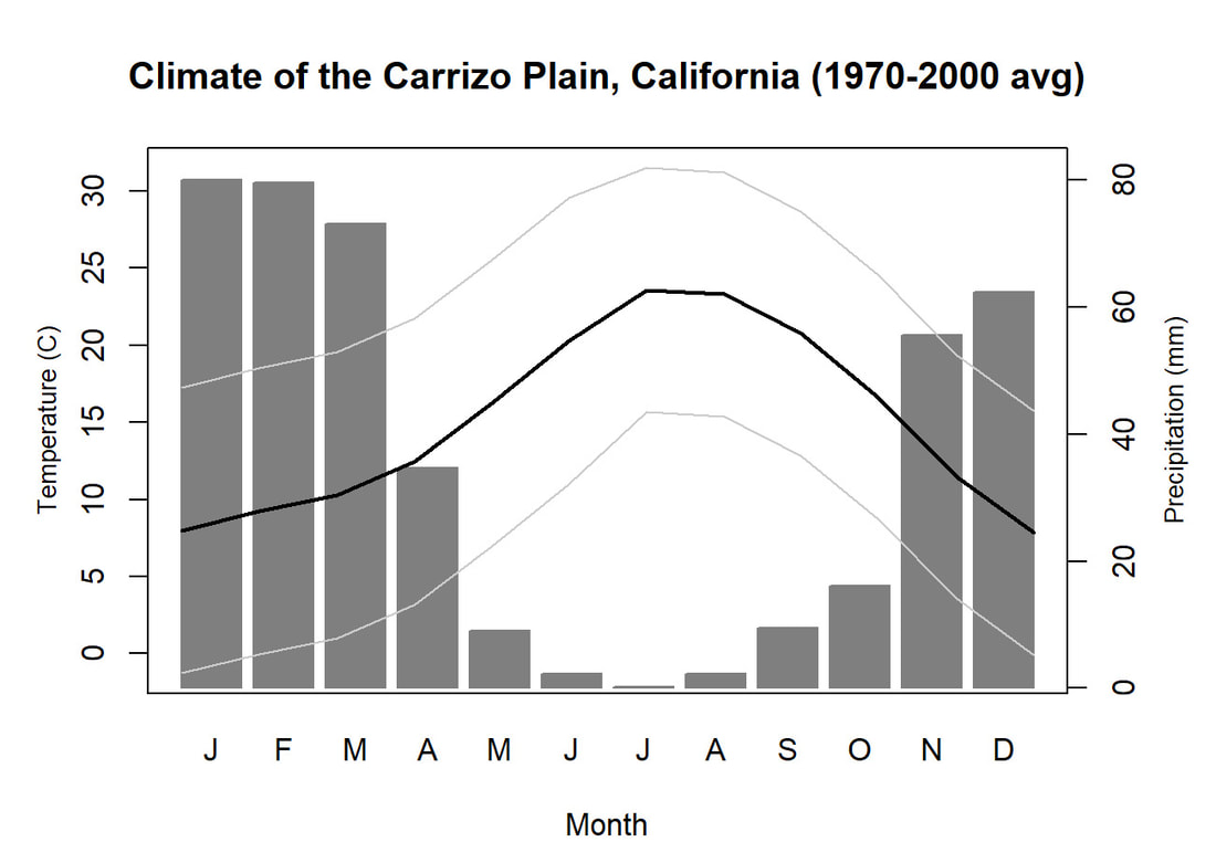 Carrizo Plain, California, climate averages for 1970 to 2000 based on worldclim data. Bars are precipiation, black line is mean temperature, grey lines are maximum and minimum temperatures. As always, there were some unexpected challenges in working through this as a class. As is typical, typos are the most common issue people have, which can be hard to spot when you're the one doing the typing. I try to pause every 5-10 minutes and check on people to see who is stuck (students have blue and red sticky notes to indicate stuck-ness, too, but without an additional instructor to help, we still take breaks). Then we ran into a few issues with the reading in of the KMZ file, with unzipping to KML (fixed in the version of the code on github), but generally for the purposes of this project we just want to create an extent object and get a general idea of the climate, so it's not essential that it is exact. We ended R Day 1 with plotting the extent on to the first average temperature raster. At the next class meeting we will pick up again there to make a data matrix and write a for-loop to read in and summarize all of the data, and make a plot. Woohoo! Leave a Reply. |
ERSAM Lab ThoughtsThis is where we occasionally post things that are not research, but more than 280 characters. If you want to know what we're working on now, this would be a good place to look. Code will be linked to here and posted on github. Archives
November 2018
Categories |

 RSS Feed