Teaching Remote Sensing in R (Days 4 & 5)

Last week and on Monday of this week we continued working in R, this time using actual remotely sensed data. This is a continuation of blog posts for days 1 (link) and day 2 (link) - I didn't include a post for day 3 because it was mostly catching up on the goals from day 2. Students have been doing awesome, however, so now we are attempting a longer set of code and introducing a bunch of new skills. The goals are (1) see how to download polygon data from AppEEARS; (2) open up a netCDF file in R (an unfamiliar file format for most of the students); (3) rasterize and summarize the MODIS data (to here on day 4); (4) write functions to map trend slopes and their significance; and (5) export that data as a KML so we can look at it in GoogleEarth (day 5). 
The code is posted here and students were given a printed out version of the 'workflow' (including instructions on how to access AppEEARS). Next time I teach this course I might have the students request their own data in advance, it just takes too long to get it back in time to request the data and work with it in the same session (my first request took about 30 min to be ready). All of this code should run on a different netCDF file, though, so they can do that on their own time if they want.
Here's the short 'accessing AppEEARS' writeup I provide (and demonstrate in class):

1. First go to appeears (https://lpdaacsvc.cr.usgs.gov/appeears/ sign in with your earthexplorer login and select ‘area samples’.
2. Name your area.
3. Zip up your shapefile (files .shp, .dbf, .prj, .shx) and then drag it in to the ‘Drop vector polygon’ box – it should show up on the map to the right.
4. Decide what you want to download (will probably need to look at the MODIS Product Table (https://lpdaac.usgs.gov/dataset_discovery/modis/modis_products_table) – also check out other things you can access via AppEEARS.
5. Pick a time period (I chose 01-01-2001 to 12-31-2015 to get a 15 year long sample).
6. Pick a product (I chose the ‘Terra MODIS Vegetation Indices’ MOD13Q1.006).
7. Pick the layers you want (I chose NDVI and ‘pixel reliability’)
8. Pick a file format (I chose NetCDF-4) and projection (I chose Geographic).
9. Submit and wait (you’ll get a confirmation email that your request has been submitted, and one when it’s done. Mine took about 30 min.)
10. Once you get the link, click on it to see the files. Kyla will show and then we take a tour of the files that are provided – NOTE: AppEEARS does not retain these indefinitely.

Once we run through all the code it will result in a figure like this one opened up in Google Earth.

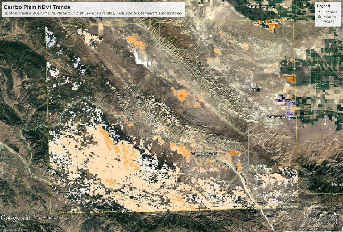Map of trends in annual maximum NDVI from 2001 to 2015 across the Carrizo Plain region. Negative trends are orange values, positive trends are purple, and transparent areas are not significant.

Overall this went pretty smoothly. Since it ran in to day 5, some students were able to fold in their own data, which was cool to see. The only major hiccup was learning that if you create a KML in R using the raster::KML function, it generates both a .kml and a .png file (I think the png holds the color info?) - and in order to look at this in Google Earth, you need both of those files to be in the same folder.
My hope is that this exercise will serve as a starting off point for students to think about other things they could map with a time series of data. What about the variance in each pixel? trends in annual minima? One thing I'm curious to try is using trend decomposition across an image (stats::stl in R), though I'm not sure how I would summarize that info to make a map that was meaningful... but it could be cool!